Business Trends
In the business of hydrocarbon production, accurate accounting of produced fluids and gases is critical from a process control, management and fiscal perspective. Since the oil and gas sector generates revenue from the production and sale of hydrocarbons, flowmeters can be thought of as the “cash registers” of the industry, as they monitor and record the quantity of product. This information is then used as the basis for custody transfer or sale. This application is true throughout the hydrocarbon supply chain, from upstream production to downstream processing and refinement, and ultimately the sale to the consumer.
Given the high specific value and throughput of most hydrocarbon production processes, heavy emphasis is placed on the accuracy of these measurements. Even minor inaccuracies can lead to significant financial exposure over extended periods of time. Ensuring accuracy and consistency over the life of the measurement system requires the operator to conduct regular maintenance, including calibration of instruments and budgeting for repair and replacement. If performed inefficiently, maintenance can be expensive. Value lies in considering the ways in which maintenance can be performed more efficiently to reduce costs.
Flowmeter development. Much of the fundamental flow measurement technology used in the oil and gas industry has been in development for hundreds, if not thousands, of years. For example, differential pressure flowmeters, which account for approximately 50% of all flowmeters in use, were first considered by Roman senator Sextus Julius Frontinus, who became water commissioner for Rome in 97 AD. Frontinus later wrote a book on the subject that considered the standardization of measurement systems and the use of pipe pressure as a means of monitoring flowrate. However, the physics behind this technique were not pioneered until the 1700s, with the scientific breakthroughs and fundamental flow theory that came from Leonhard Euler, Daniel Bernoulli, Leonardo Da Vinci and others.
Many flowmeters that were developed based on these fundamental principles are still heavily relied upon within most industrial sectors, including oil and gas. These devices are often classed as “traditional” flowmeters. Examples include turbine flowmeters and differential pressure devices, such as orifice plates and Venturi tubes. Despite their age, these devices remain popular because they are a well-understood technology developed over years of research. Coupled with their inherent mechanical simplicity, these devices enable the achievement of a very high degree of accuracy.
The defining feature of traditional flowmeters is that energy is removed from the flow stream through the impingement of the flow on the mechanical components or body of the flowmeter, regardless of the fundamental principle of operation, be it differential pressure, turbine or vortex, etc. For example, a differential pressure meter throttles flow to create a measureable differential pressure, resulting in some degree of unrecoverable pressure loss within the system. In this sense, “traditional” technologies have the inherent weakness of being inefficient.
Furthermore, mechanical components that interact with the flow can be problematic in many applications. For example, systems where a flow stream contains contaminants, such as solid particulates or small amounts of a secondary fluid phase, can result in erosion or mechanical wear, thereby adversely affecting the performance of the device. The pressure loss associated with such devices can also be a serious problem and is undesirable from a process perspective, resulting in cavitation, reduced flow or other issues.
With the advent of modern electronics, the long-established technology behind traditional meters is being supplanted by new flowmeter types and technologies. The oil and gas sector is just one of the industries benefiting from recent, rapid technological advances.
The key advantage of modern technologies over traditional flowmeters is that, in contrast with traditional flowmeters, which work by removing energy from the flow stream, modern technologies achieve flowrate measurement through the addition of energy to the flow stream. For example, ultrasonic flowmeters (USMs) work by passing ultrasonic pulses between transceivers mounted in the pipework, and use the pulse latency to infer flowrate. Since these techniques do not require the removal of energy from the flow stream and often do not interact with the flow, the technology is generally considered “non-intrusive”—i.e., the device does not need to impinge on the flowstream to work.
Flow measurement in the real world. Flowmeters are principally designed to return a measurement of the flowrate. In a laboratory environment, this can be achieved with a very high degree of accuracy if the correct meter is selected for a given application. The problem is that ideal scenarios are hard to find in reality. Poorly designed pipework, the lack of upstream and downstream pipe lengths or flow conditioning, contamination, under-maintained facilities and many other factors can impede flowmeter accuracy.
Where it is necessary to maintain a required level of accuracy, as in the case of fiscal or process management and control applications, regular system maintenance is essential. When a flowmeter is purchased, it should be calibrated at a range of conditions that mirror, as closely as possible, the operating envelope of the system in which the device will be installed. For gas flow applications, these calibrations include aligning the operating conditions (namely through the Reynolds number) and other application parameters, such as pressure and temperature.
The problem is that, over time, the performance of the device will drift, resulting in higher measurement uncertainty. This drift can be caused by a range of factors, such as a shift in system operating conditions or the composition of the measured flowstream. Erosion or mechanical wear can also influence certain devices, particularly intrusive flowmeters, such as turbine meters, where bearing wear can subtly shift meter response over time.
The issue with drift is that it may not always be apparent that it is happening, and the rate of drift may be difficult to determine. To combat this problem, a maintenance schedule is normally developed that includes regular meter calibration to compensate for drift. This schedule includes periodic calibrations of both the primary flow sensor and any associated secondary instrumentation.
Approaches to calibration. Traditionally, most operators perform meter calibrations on a time-based calibration schedule, and therefore incur an annual or biannual expense, in addition to the inconvenience caused by removing the flowmeter in the event that the calibration is not performed in-situ, such as during a system shutdown.
However, time-based calibration scheduling is just one possible approach to system maintenance, as numerous calibration scheduling methodologies are available. Three of the most common approaches are summarized:
- Time-based calibration: Device calibration based on a specified time interval. Factors such as instrument type, operating conditions, measurement application and manufacturer recommendations are some of the factors that are considered when selecting a calibration interval.
- Risk-based calibration: Calibration scheduling based on the degree of financial exposure caused by calibration drift over time, weighed against the cost of calibrating and maintaining the device for a given calibration interval.
- Condition-based calibration: The use of diagnostic data acquired from the device or measurement system, either through post-processing of the primary measurement data or as secondary data, which can provide qualitative and, in some cases, quantitative insight into the health of the measurement system, as well as indicate deviations in the performance of that device or system.
One flaw of a time-based calibration scheduling system is that it pays little to no attention to whether the meter actually needs to be calibrated. In some cases, the rate of drift of the measurement system may be more severe than estimated when scheduling the calibration. In other cases, there may be no need to calibrate as frequently as the schedule demands. In either case, it is likely that the calibration schedule is not optimal and may be costing the operator money. If calibrations are performed too infrequently, then the degree of financial exposure associated with the mismeasurement may exceed acceptable limits. If the calibration is performed too frequently, then the operator may be generating extra work and expense associated with unnecessary maintenance.
To address the weaknesses of time-based calibration schedules, the risk-based and condition-based approaches are increasingly used as the bases for calibration scheduling. The risk-based approach attempts to characterize the risk associated with a given measurement system; in a fiscal measurement system, the objective is to trade off maintenance costs with financial exposure. The basic premise is that an optimal length of service exists at which the meter should be calibrated. This service length depends on the rate of drift of the meter, which is influenced by many factors, including meter type, operating environment, measurement application and the maximum permissible exposure.
In fiscal metering applications, where the measured fluid has a relatively high associated value, mismeasurements can be costly. This leads to the concept of financial exposure, which results from the measurement uncertainty that is inherent in all measurement systems. If the flowrate and fluid value are taken into consideration, then the financial exposure is the potential cost associated with the possible mismeasurement of that flowstream. The magnitude of the financial exposure within a system corresponds to the level of drift of the meter.
At some point, the financial exposure exceeds a predefined acceptable level. However, it is also necessary to consider the cost of maintenance, which is not insignificant and comprises the costs of calibrating the device, making repairs, maintaining staff and taking into account facility downtime. It is logical that the less maintenance that must be done on a system, the lower the costs. One of the key variables in terms of maintenance costs is the frequency of calibration; i.e., if the calibration period can be extended, then the average cost is reduced. The question then becomes: How do we evaluate the optimal calibration period?
The optimal time to calibrate a meter can be thought of as the point at which the financial exposure equals the maintenance cost. The key to establishing the time at which this occurs lies in an understanding of the way a meter’s performance deteriorates with time. With every successive calibration or verification for a given device, data becomes available that allows the magnitude and rate of drift to be evaluated. Using historical data, it is possible to infer trends that describe drift characteristics for that device. This information forms the basis of a financial exposure model, which allows the time-dependent financial exposure to be evaluated. It also enables a trade-off between financial exposure and maintenance costs, as well as the determination of the optimal calibration period.
The alternative approach to risk-based calibration scheduling is the condition-based method. With the advent of modern electronics and computers, it is possible to extract a significant amount of data from flowmeters over and above the basic information pertaining to the flow measurement itself. This is particularly true of sophisticated, modern flowmeters, which rely on advanced electronics. Data output from flowmeters can be post-processed to provide insight into the performance of the meter.
An example of this post-processing method is the ability of most USMs to return the speed of sound, in addition to the axial velocity of the flow. The advantage of this is that the speed of sound for a fluid or fluid mixture at a given set of operating conditions can be accurately measured. With this information, it is possible to track deviations in fluid composition, which may have a knock-on effect on the estimated flowrate. A summary of the speed of sound and other diagnostic parameters is given in Table 1. This large range of metrics provides the ability to diagnose problems that could affect measurement accuracy.
 |
Experimental work also allows some traditional flow measurement devices to be used in this way. Differential pressure meters can be made to work in wet gas flow conditions, where correlations based on experimental research can allow the gas volume fraction (GVF) to be established from differential pressure ratios measured at different points within the device.
This type of diagnostic capability, in addition to the ability of some meters to self-diagnose internal mechanical or electronic issues through condition monitoring, can provide substantial insight into the operation of the flowmeter. It can also provide confidence that the meter is functioning correctly. Therefore, when a meter begins to underperform or deviate from its standard performance, it is possible to recognize and evaluate the nature of the problem. This process can often be carried out before a problem fully develops. In other cases, such problems would go unnoticed for some time before developing into more serious issues. As such, condition monitoring makes it possible to take action to mitigate potential problems ahead of time, and to use preventive measures such as maintenance and calibration. Nevertheless, diagnostics alone are not enough to ensure flowmeter accuracy over long-term use, and calibration remains an essential part of flow measurement system maintenance.
The increasing availability and sophistication of modern meter diagnostics makes risk- and condition-based calibration scheduling possible and offers the advantage of increased operational efficiency. The inherent weakness in the existing system of calibrations based on a set interval is that it does not necessarily take account of the condition of the meter. It also does not take into account whether the meter has been subject to a statistically significant degree of calibration drift that is likely to impinge on the ultimate accuracy of the measurement and the resulting financial exposure.
This means that the operator could be performing calibrations with unnecessary frequency and incurring the costs that come with calibration while the meter is drifting or deteriorating at a higher rate than anticipated, resulting in increased financial exposure. The problem is that without considering the financial exposure associated with drift or with using diagnostics and condition monitoring, the operator does not know if either of these situations is occurring.
In principle, the ideal calibration strategy is a combination of these approaches—qualitative, “condition-based” diagnostics data used in conjunction with statistical modeling, based on data from historical calibrations, to drive efficiency, reduce costs and maintain accuracy.
Despite the benefits of using these modern approaches to calibration scheduling, many operators still rely on time-based scheduling. A number of reasons highlight why this may be the case; the simplicity of time-based scheduling, lack of training, outmoded apparatus, lack of budget and organizational inertia may be factors for why some operators have not yet embraced this new mindset. It is clear that many operators will need to adopt a new approach to flowmeter calibration scheduling before risk- or condition-based calibration becomes the norm over time-based calibration. GP


Comments