
Optimization of cryogenic NGL recovery plants using dynamic online process simulation—Part 2
This article—a continuation of the first installment published in the August issue of Gas Processing & LNG—discusses DCP Midstream’s approach to plant optimization using dynamic process models and present some actual operating examples demonstrating the benefits, such as:
- The continuous optimization of plant performance, accounting for changes in feed conditions, residue sales pressure, ambient temperature and other factors
- Allowing for more rigorous process modeling while avoiding convergence issues commonly encountered with similarly complex steady-state models
- Models that can include additional engineering data that answer more complex what-if analyses
- Real-time, multi-plant optimization via rigorous modeling of plant limitations, particularly the impact to NGL recovery as a function of plant throughput
- Taking advantage of short term market price swings since the simulation enables immediate identification of plant limitations for a new operating mode.
Thermosiphon loop modeling. Many NGL recovery plants operate with one or more reboilers for the demethanizer column that utilize a thermosiphon configuration. A properly designed thermosiphon loop enables flow through the reboiler and back to the tower without the use of a pump or other rotating equipment. A once-through thermosiphon operates on the principle that the density in the reboiler feed line is higher than the density in the return line due to partial vaporization in the reboiler. Therefore, the driving head (h1–h2 in FIG. 5) can overcome the pressure losses in the piping and the reboiler.
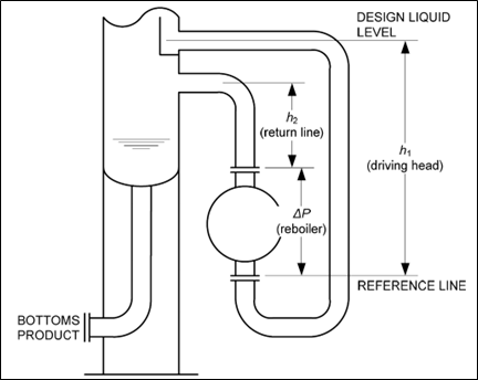 |
| FIG. 5. Schematic of a thermosiphon reboiler circuit. |
The design of these loops must consider the available pressure differential (including the outlet vapor fraction and the geometry/elevation of the piping), as well as the resistance of the heat exchanger and piping.
If the density difference is low, due to low vaporization or during startup, operations can use lift gas (typically dry residue gas) in the return line to lower the return density and establish enough driving head to start flow through the reboiler. Low vaporization occurs at low feed gas rates because, in cryogenic plants, the hot side duty of the reboiler is provided by feed gas. In addition to potentially stalling the reboiler, low feed rates can also result in an unfavorable flow regime in the return line. Ideally, the flow regime is continuous (bubble flow or annular), but at low feed rates intermittent (slug) flow is almost unavoidable.
A common problem plaguing many gas plants, particularly those with braised aluminum heat exchangers (BAHX) reboilers, is a malfunctioning thermosiphon loop. Because of their design, they are particularly susceptible to deviations in flowrate and composition and to exchanger fouling. If the flowrate is reduced below design, the outlet flow regime can change such that there are transient conditions of 100% liquid in the return line. This causes the pressure differential to approach zero, and flow through the thermosiphon ceases. If the exchanger is fouled, its resistance to flow increases. At the same differential pressure, the flow decreases, though the flow rate from the demethanizer has not changed. As a result, the height of liquid on the supply line increases, until at a certain point, the liquid height reaches the top of the piping and begins to flood the draw-off tray for the reboiler. The draw-off tray may overflow, resulting in lost heat integration, difficulties meeting NGL specificationsand potential flooding in the tower itself.
In a dynamic model, the thermosiphon loop can be rigorously modeled, including the draw-off tray, piping configuration, exchanger pressure drop/flow capacity and elevation differences. The effect of changes in gas composition and rate can be evaluated directly while the simulation is running. In a steady-state model, this can only be accomplished with several controllers/adjusts and additional calculators, but these often cause model instability and will still be less accurate than modeling in the dynamics engine.
Thermosiphon loop modeling: Example. A DCP Midstream plant with multiple BAHX thermosiphon loops in operation suffered from regular exchanger fouling and tray flooding. This issue was risking steep fines for off-spec NGL (maximum C1 content) on a recurring basis.
This plant operated with a variable inlet rate. As a result, the amount of tray flooding that occured is variable in a non-linear fashion. The plant’s dynamic model was used to evaluate the thermosiphon loop using the known piping geometry for the supply and return lines and the exchanger’s design flow resistance. This analysis showed that if all the liquid were flowing through the thermosiphon, the flow regime was in the desirable region across the range of operating flows for the plant and no tray flooding should occur. Therefore, the observed problems must be due to heat exchanger fouling. This was verified by operational experience from the times in which the exchanger was taken out of service and cleaned, where the small flow passages were found to be partially blocked.
Closing the heat and material balance in the simulation for the plant during stable operations enables accurate estimation of the exchanger flow resistance/capacity. DCP Midstream’s experience is that the model remains reasonably accurate when extrapolated beyond the calibration point. This plant had been operating at ~100 MMsft3d for some time, and changes in the field required consideration of increasing the inlet rate of this plant. There were multiple options for routing the incremental gas;however and given that the bottom reboiler thermosiphon loop had begun to malfunction again, the plant’s ability to hit the NGL product specifications were in question at these higher rates.
Using the model that was calibrated for the current flow resistance of the bottom reboiler, sensitivity studies were completed, including the impact to plant performance as a function of inlet flow rate. The results are presented in FIG. 6.
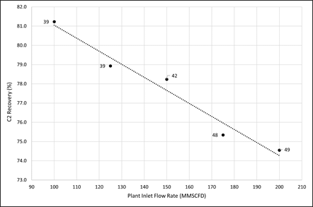 |
| FIG. 6. Impact of changing plant inlet rate on maximum C2 recovery for a plant with flooding reboiler draw tray (required reboiler temperature annotated in °F). |
The simulation was able to quantify the decrease in maximum C2 recovery for the plant as the inlet rate increased. For all cases, the operating pressure of the demethanizer remained constant. As the flowrate increased, the load on the refrigeration system (which is modeled rigorously) increased, and the impact from the flooded bottom reboiler draw tray increased. The combination of these two factors required an increase in the temperature control set point for the bottom reboiler return to maintain NGL spec—the required temperature is indicated as a data label for each point.
By completing this analysis for the plant, as well as the other plants in the area at which the incremental gas in the field could be processed, a holistic view of the system can be taken. It may not be advantageous to process all the incremental gas at this plant due to its decrease in performance. Further, the results (as well as the model that will run continuously in the background) provide guidance to the operator on what temperature the demethanizer reboiler return should be controlled tomaintain the NGL C1 specification, avoiding potential off-spec fees.
Control valves and control loops modeling. In steady-state simulations, including process controllers that are representative of actual plant control is often very difficult. These controllers add more complexity, increase the convergence time and, in some cases,make convergence impossible due to the way some unit operations are required to be specified. Additionally, given that one of the goals of the simulation models is to provide guidance to an operator on how to optimize the plant, having a simulation philosophy that is consistent with real controllers in the plant is beneficial.
The inclusion of control information often complements the other items previously discussed. The following are examples:
-
Turboexpander controls. Some plants operate with the expander near the high-high shutdown speed and use a speed override to limit the guide vane opening such that a target speed is not exceeded. At higher flow rates, the JT valve will start to open. Accurately quantifying the maximum expander capacity has significant impact on predicting plant performance. Experience has shown that including this limitation in steady-state models is arduous.
Some plants operate with the brake compressor surge valve partially open. This limits the boost pressure generated, as well as affects the speed of the unit. By including this effect, the impact to plant residue compression, demethanizer pressure and expander speed (if this is a bottleneck) can be calculated.
-
Cryogenic plant recycles and compressor recycles. When coupled with rigorous compressor modeling, these controllers can provide recommended set points to an operator. For instance, at what speed should inlet and residue compressors be operated to maximize recoveries and minimize energy usage? Similarly, if a low suction pressure recycle exists, the model will only allow the performance to increase to a certain point and additional compression will not have any effect.
-
Cryogenic plant inlet split controllers. Most cryogenic plants split the feed gas at the inlet to the cryogenic plant using one or two control valves. Part of the feed goes to provide heat to the demethanizerreboilers, and the balance is sent to other unit operations (usually a gas/gas heat exchanger). To close the heat and material balance for the plant, as is required for calibrating the performance of heat exchangers and other items, determining the relative flow split is critical. Some plants have flowmeter(s), but these are not always accurate, and other plants do not have them at all. The nature of the pressure/flow solver will calculate the relative flow based on the pressure at the inlet of the split, the pressure downstream of the split and the flow resistance of the equipment between. By inputting the control valve information for each stream at the split (Cv curve at a minimum) and additional information for the other flow-restricting elements in each stream, the flow can be estimated. These flow-restricting elements can include rigorous modeling of heat exchanger geometry/K-factors, piping, orifice plates, etc.
An additional benefit to this type of modeling is that it enables an accurate prediction of plant limits. A steady-state simulation may allow the flow to a reboiler pass to be a very small fraction of the inlet flow to operate the reboiler at as low a temperature as possible. However, in practice, there usually are minimum stops on the control valves, and this represents a limit for the optimizing simulation.
-
Centrifugal pump minimum flow recycles and discharge pressure control valves (runout). Many centrifugal pumps use a control valve to maintain a minimum continuous flow through the pump. Similarly, a valve is often placed on the discharge to maintain level control, a minimum discharge pressure to prevent runout, etc. These control schemes—coupled with the fact that many pumps in a gas plant operate at multiple speeds—makes the operation of these units dynamic. While in many cases, capturing this detail is trivial to modeling the performance of the plant, for some designs, it is critical. Some pumps flow cold NGL to a heat exchanger to cool the feed gas stream—this now-heated NGL can then be recycled via a minimum flow controller back to the bottom of the demethanizer. In this configuration and others like it, the amount of liquid flow through the system can have an impact on the performance of the plant and is also tied to the number of pumps that are running and the sales line pressure for the NGL. While this system can be modeled in a steady-state simulation, it requires multiple controllers and typically leads to model instability and convergence issues that preclude its use for models that run continuously and unsupervised.
-
Control valve sizing and controller tuning. By including control valve data, one can determine if an installed valve is over/undersized. This can even be coupled with accurate vessel/equipment sizing and real PID tuning parameters to show how controllers/valves impact process stability. For instance, if a relatively small vessel is paired with an oversized valve and an aggressively tuned level controller, this can lead to large variations in liquid outflow, impacting downstream heat integration. The simulation can then be used to provide a preliminary analysis on what size valve may be appropriate or if tuning parameter changes may help.
Control valve data (e.g., Cv curve, FL curve, xT curve) can be included in most steady-state models. However, when used in dynamics modeling, combined with the pressure/flow solver engine and the rigorous modeling of other equipment, it becomes a much more powerful tool for predicting plant performance.
Example 2: Optimizing a fractionation train. A DCP Midstream plant consists of an NGL recovery cryogenic plant feeding a fractionation train that produces purity ethane and propane products. This fractionation train can be bypassed partially; the Y-grade is sold with the bottoms product from the depropanizer tower. However, the goal is to produce as much purity product as possible, as these streams produce higher margins than selling the components as part of a crude NGL stream. Generally, the capacity of the fractionation train is limited by the capacity of the deethanizer reflux condenser, which is a total condenser. Cooling is provided by a propane refrigeration system. The deethanizer pressure is controlled using a hot vapor bypass. A process flow diagram (PFD) of this system is shown in FIG. 7.
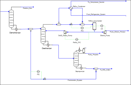 |
| FIG. 7. PFD with NGL recovery and fractionation train. |
During periods of high flowrates or high ambient temperatures, the available cooling duty from the propane refrigeration system may be derated significantly. This results in the condenser bypass valve closing fully while the pressure continues to climb. Eventually, the pressure will be controlled by flowing purity ethane vapor to the residue gas line. This is undesirable, as this is the lowest margin sales point for the ethane. To avoid this, the operator attempts to keep the reflux condenser bypass valve open slightly to be in control but closed as much as possible to maximize feedrate to the fractionation train.
Complicating matters is that as the overall NGL recovery level in the demethanizer is increased, the NGL C1 content increases. The C1 component significantly increases the vapor pressure of the purity ethane product even at relatively low levels, which increases the required duty on the reflux condenser and exacerbates any deficiencies in that system. Altogether, maximizing the performance of this system is a function of the following:
- The NGL recovery level in the cryogenic plant (and the associated C1 content of the feed to the fractionation train)
- The flowrate of the fractionation bypass
- The ambient temperature (affects available horsepower and cooling duty for the propane refrigeration system)
- The feed rate to the plant/fractionation train.
The engineer must optimize all these parameters simultaneously to produce the maximum amount of purity products possible, while minimizing fractionation bypass and eliminating any ethane vapor from flowing to the residue gas stream. The crude NGL stream must also comply with a maximum NGL C1 specification, which may be breached at high levels of fractionationtrain bypass.
The dynamics engine is well suited to solve this problem. The condenser and its bypass valve can be rigorously modeled to ensure accurate representation of the unit. This includes a rating model on the exchanger and ISA sizing calculations on the control valve. The optimization can then take place unsupervised and in real time, with the following philosophy:
- The ambient temperature data is input to the simulation as a parameter for the propane refrigeration system. This may include the condenser operating pressure, an approach to the refrigeration condenser temperature and/or a derate on compression horsepower.
- The NGL recovery level in the cryogenic plant is increased until the position of the condenser bypass valve is 20% open (minimum for stable operation). The recovery controller must also operate on a selector block that limits the C1 content of the purity ethane below the maximum product specification.
- The simulation begins to bypass NGL around the fractionation train to allow for higher NGL recovery in the cryogenic plant without exceeding the available duty of the reflux condenser. This flow controller also operates on a selector block that limits the C1 content of the crude NGL product below the maximum product specification.
- All this optimization occurs simultaneously while also optimizing the fractionation operation in the traditional manner, including managing reflux flows and reboiler temperatures on both columns to maintain purity product specifications and maximize production.
The simulation includes control valve data from other controllers in the system, as well as the centrifugal pump curves and other data to ensure that all optimized process values are physically achievable. This level of detail and rigor is unachievable in a steady-state simulation while maintaining the ability to converge reliably with ever-changing inputs. By providing process targets to the operations team, it ensures that the plant is always operating in the way production rates are maximized, accounting for changing performance as feed rates, composition and ambient temperature changes occur.
Conclusions and future opportunities. The following are benefits to the company and the engineer, along with future opportunities.
Benefits to the company. As DCP Midstream has increased the capability of its Integrated Collaboration Center (ICC) and the engineering support therein, the group has increased the rigor of its process simulation capabilities. Replacing the original steady-state models that included ever-changing plant performance data and ran hourly, the current models are dynamic process models that contain much more engineering data and continuously provide operational guidance and feedback to operations teams constantly.
In addition, the dynamic models allow for a greater amount of engineering data input, along with much improved model stability and convergencevs. complex steady-state models. As a result, the engineers can more easily provide precise answers to what-if analyses. These include the types of technical questions regularly asked about midstream gas plants, including:
- How will changing inlet gas composition, feed rate or other external factors affect plant performance and what are the potential bottlenecks in the plant?
- Determining if changing the number of compressors, pumps, etc., in operation is possible, and how will affect plant performance?
- Quantifying how a change to a control scheme or set points will impact plant performance, and how will the existing control valves in a system may manage this change?
By continuously providing optimum plant guidance to operations and by having a rigorous process simulation that accurately predicts plant performance across a wide range of conditions, DCP Midstreamhas been able to increase plant profit margins, maximize asset profitability through optimum plant loading and reduce operating expense. It allows the company to react quickly to changes in market/pricing conditions, allowing every plant to capture the maximum value every day. The increased accuracy of the simulations enables DCP Midstream to go past the low-hanging fruit of optimization (the 80/20 solutions) and capture more of the remaining benefit. In the competitive midstream industry where pricing, cost control and reliability are essential, this incremental benefit can have a significant impact.
Benefits to the engineer. With limited engineering resources, prioritization of tasks must occur. Because of this, the bulk of time is spent on day-to-day activities to keep plants safely running, leaving little time for plant optimization. With traditional plant process models, answering difficult technical questions and what-if analyses requires the combined use of a process simulator, vendor software for equipment performance and control valve information, and significant amounts of hand calculations and iterative processes. While the dynamic models described in this article require more up-front effort to construct vs. a more traditional steady-state gas plant model, they greatly reduce the effort required for the engineer to complete optimization and troubleshooting analyses. The wealth of data generated from the continuously running dynamic simulation also enables easy maintenance of the models, such that for each plant there always is an accurate process model available.
By reducing the amount of time spent solving each technical problem, more problems can be solved. Plant optimization, optimal routing of field gas and operations troubleshooting exercises using simulations can be completed daily, if necessary. The continuous operational targets provided allow operations to essentially have engineering support at any hour of any day.
Future opportunities. In addition to the increased engineering rigor incorporated in dynamic models and their better performance, the models also allow for quantitative analysis of time-dependent events. In recent years, for example, thermal stress failures of BAHX have received much attention, with manufacturers providing strict guidance on maximum allowable temperature rates-of-change. With frequent changes in feed rate or composition and desired ethane recovery to respond to market conditions, the operating temperatures of the cryogenic plant may have to be regularly adjusted, and these changes must be completed in a controlled manner.
The dynamic models can be used to provide guidance to the operations teams on how best to make these plant changes to minimize the risk of unacceptable thermal stress. Because the dynamic simulations can model time-dependent trends of temperatures, they may help provide this guidance. In addition to how quickly to change set points such as the bottoms temperature on the demethanizer, they may provide insight on which variables are best to change first. For example, is it better to unload the refrigeration system and then increase the demethanizer reboiler temperature or vice versa?
The experience that DCP Midstream has gained while setting up the infrastructure for the continuously running dynamic models of its cryogenic plants has resulted in valuable insight in plant operations and bottlenecks. Considering these benefits, dynamic simulations for other parts of the processing plants and field operations will continue to be developed. GP
Jake Carrier has been a Process Engineer in DCP Midstream’s operational support and optimization group (ICC) for 5 yr, where he provides technical support for gas plant and field operations teams. His previous experience includes 5 yr working in engineering, procurement and construction as a Process Engineer on projects, including upstream and midstream facilities, sour gas and supercritical carbon dioxide. Mr. Carrier is a graduate of the chemical engineering program at the University of Colorado in Boulder.
Sjoerd Hoogwater heads the ICC Engineering group at DCP Midstream in Denver, Colorado. He has more than 30 yr of experience in the oil and gas industry. He joined DCP Midstream in 2019 to help expand their process technology and optimization capabilities. Mr. Hoogwater earned an MS degree in chemical engineering from Eindhoven University of Technology in The Netherlands.


Comments