Optimization of cryogenic NGL recovery plants using dynamic online process simulation

DCP Midstream actively adjusts the operation of its cryogenic natural gas liquids (NGL) recovery plants based on real-time comparison of plant performance with dynamic process simulations. A dynamic process simulation of each plant is continuously running in the background, providing operators with guidance for process conditions. The simulations provide valuable insights into operations, bottlenecks, equipment health and optimization opportunities.

This article details DCP Midstream’s approach to plant optimization using dynamic process models and presents actual operating examples demonstrating benefits such as:

• The continuous optimization of plant performance, accounting for changes in feed conditions, residue sales pressure, ambient temperature and other factors
• Allowing for more rigorous process modeling while avoiding convergence issues commonly encountered with similarly complex steady-state models
• Models that can include additional engineering data that answer more complex what-if analyses
• Real-time, multi-plant optimization via rigorous modeling of plant limitations, particularly the impact to NGL recovery as a function of plant throughput
• Taking advantage of short term market price swings since the simulation enables immediate identification of plant limitations for a new operating mode.

DCP 2.0 initiative. Identifying that the oil and gas industry at the time (and particularly the midstream gas processing industry) was lagging other industries in technology adoption, DCP Midstream launched its DCP 2.0 initiative in 2015. The premise of the initiative was to leverage new technology and processes, leading the way in modernizing the midstream sector. The primary strategic objectives of this initiative were to:

1. Achieve real-time optimization and decision-making in assets
2. Use real-time data to make more strategic business decisions, increasing reliability/runtime and improving margins
3. Improve asset reliability and safety
4. Increase efficiency through automation, create digital platforms and create a modern workforce with a culture of innovation and agility
5. Improve safety and decrease emissions through enhanced process monitoring; utilizing predictive analytics to improve asset maintenance.

The initiative included the creation of an Integrated Collaboration Center (ICC) in 2017 to bring together key groups from across DCP Midstream for regular cross-functional engagement to achieve the strategic goals of DCP 2.0. These groups included operations (local and remote), engineering (local and corporate), commercial, finance and gas control. This enabled the linking of key data sources, including supervisory control and data acquisition (SCADA) and distributed control system (DCS) information, financial/contractual data, real-time product pricing and engineering data.

The ICC includes monitoring and optimization of 35 plants and their associated gathering systems, remote operation of 25 plants/boosters, gas control for most of DCP Midstream’s gathering systems and residue gas sales points, as well as commercial, financial and engineering support. This organization creates a unique opportunity to see large regions and the company as one entity rather than many individual assets operating independently. With this centralized view, even relatively small gains can be extrapolated across many assets and substantial gains may be realized.

Process simulation for midstream gas plants. Prior to the establishment of the ICC, process simulations were used at DCP Midstream in similar fashion to many other midstream operating companies at the time. The simulations were used only intermittently as needed to perform what-if analyses. These would include emissions modeling, evaluation of potential projects/equipment additions or to provide high level guidance to operations, such as changes in operating mode (e.g., ethane recovery vs. rejection).

The steady-state process simulation models usually included little engineering data and were often oversimplified for ease of use and shorter convergence times. These included:

1. Fixed process outlet temperatures for refrigeration systems: This value would often be based on a heat and material balance or design value. At best, it would be based on recent historical values. In either case, this fails to capture the impact of changing plant conditions (e.g., the number of operating units) on the performance of the refrigeration system.
2. Fixed process temperature for most heat exchangers: Again, this would be based off recent operating data at best, but also failed to capture dynamic plant performance across varying conditions. In some cases, the heat exchangers would be specified using UA values. This is a more rigorous method for quantifying performance that better predicts changing exchanger performance across varying conditions. However, the UA values for a given exchanger can change significantly over time, so use of this method requires regular re-evaluation of the values used. This was typically not done with high frequency in these models at the time.
3. Fixed operating pressures based on historical operating data: This was most used for the cryogenic plant inlet pressure and the operating pressure of the demethanizer. Given that the demethanizer operating pressure is one of the most important operating parameters for the facility, quantifying it appropriately is key to optimization exercises.
4. Fixed efficiency and horsepower specifications for compression in lieu of more rigorous modeling: This is a common limitation of simple steady-state plant models. At best, the suction pressure of a unit would be lowered until the design horsepower of the machine was calculated, and this was taken to be maximum performance. In practice, however, determining maximum compressor performance is a complex problem that must consider many things beyond the maximum horsepower of the driver.

Because of the nature of these models, impacts to plant performance based on feed rate/composition changes, ambient temperature changes, equipment count, etc., were difficult or impossible to accurately quantify. Not only were the models not run with high frequency to allow for providing operational guidance, but they were ill-equipped to perform complex what-if analyses.

While these models were fit-for-purpose at the time, the initiatives of DCP 2.0 called for more advanced process modeling to achieve stated goals of real-time optimization.

Data gathering and ICC plant screens. As part of the DCP 2.0 initiative, a database of operating information was developed using a proprietary data management platforma. This system allows continuous collection and organization of large amounts of operating data, including:

• Data from gathering systems that use SCADA
• Data from plant control systems that use DCS or Wonderware systems
• Weather data
• Compressor analytics data (derived data from raw source data)
• Operator rounds data (e.g., amine strength).

This collection of data enabled employees across the company and in any discipline to easily access historical and current operating data using custom dashboards, monitoring tools and key performance indicator (KPI) screens.

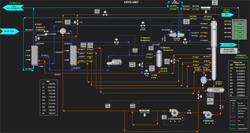
One of the platforms used commonly in the ICC were plant screens (FIG. 1). These screens present a process flow diagram- (PFD-) style view of a processing plant, along with key operating data from the proprietary data management platforma. The screens contain KPI tables which allow for monitoring of parameters such as NGL recovery, product specs and plant throughput. The screens allow easy access for data trending and are available to anyone within DCP Midstream.  

FIG. 1

The plant screens enabled the ICC to not only monitor current plant performance, but also display values from a process simulation for comparison. This would enable engineers, operators and other support groups to better understand in real time if the plant was achieving its operational targets (via the KPI table).

An example of the cryogenic portion of a plant screen is shown in FIG. 1. Values in white are actual data which is linked to the plants’ control system. The yellow numbers alongside are the values outputted continuously from the simulations. The screens can be viewed historically, which allows a complete overview of the plant conditions at any time in the past. Most systems are limited to trending several historical data points at a time, and in many cases are not particularly user-friendly.  

The simulations run continuously in the background as digital twins, receiving inputs from the proprietary data management platforma such as inlet composition, feed rate, inlet pressure/temperature and other key inputs, as required. The simulations are configured such that they target an optimum condition as determined by the engineer. These may include:

• An ethane recovery mode simulation in which the NGL recovery is increased until the maximum NGL product specifications are reached
• An ethane rejection mode simulation in which the NGL recovery is decreased until the maximum residue gas heating value is achieved.

Other limitations to operating modes may be included in the simulation as discussed later in this article.

If a discrepancy exists between plant KPI values and those predicted by the optimized simulation, comparison of outputs from the simulation with actual operating data can provide an explanation. For example, perhaps the bottoms temperature of the demethanizer column is higher than is necessary to achieve NGL product specifications. This provides a basis for discussion with the operations team on an actionable change, in this case, the set point of the bottom’s temperature controller. As the program matured and trust in the simulations increased, this discussion became unnecessary in most cases, and a culture of driving plants toward operating targets on a continuous basis was created.  

Even in instances where the simulation may have provided an infeasible target, valuable insight may still be gained. To continue the example, it may be learned upon discussion with facility operations that the NGL product analyzer, which has been demonstrated to be very reliable, is showing that the current temperature set point is yielding product near the maximum specification. In this case, reducing the temperature controller set point to match simulated values would yield off-spec product. With this information, the engineer can then perform an offline analysis to understand why the plant is unable to achieve the predicted performance. This analysis could then conclude that the draw tray for the bottom reboiler is in a flood condition, bypassing some liquid product around the reboiler and requiring a higher operating temperature in the bottom of the column to stay on-spec. Now, a limitation of the plant has not only been identified, but fully quantified. This performance degradation can then be tracked over time, and a financial impact can be determined.

With this kind of real-time, in-depth performance data gathered over time across multiple plants, multiple assets and ultimately across the company, better informed business decisions can be made. These decisions can pertain to feasibility of proposed new gas packages, determining whether a plant may continue to operate without an amine system or refrigeration, or optimum gas routing in an under-utilized asset where gas routing is flexible.

The development and maintenance of these simulations is one of the core functions of the ICC engineering group. DCP Midstream’s operations teams have access to these screens, which allow operators to get engineering feedback on their plant at any time all year long. Ultimately, the success of such a program hinges on the quality of the simulation providing the guidance and capturing the bottlenecks.  

ICC steady-state simulations. The first iteration of the process models developed for the plant screens were steady-state models like their predecessors. These models ran as frequently as possible, based on convergence time and the maximum number of simulations the server computer could run simultaneously. This generally led to new simulation data being provided to the operator about every hour.

These simulations contained more engineering data than the legacy models, including:

• Use of UA specifications for heat exchangers in lieu of approach temperatures or fixed outlet temperatures.
• Demethanizer and other distillation column tray efficiencies adjusted based on operating data
  • Legacy simulations often used typical efficiencies or equilibrium stages
• Turboexpander and brake compressor efficiencies adjusted based on operating data
  • Legacy simulations often used design efficiencies from datasheets
• Liquid carryover from the demethanizer overhead and demethanizer tray flooding included as determined from operating data, composition data, and the plant heat and material balance
• Pressure drops through heat exchangers or other equipment, adjusted based on operating data
• Refrigeration system performance used compressor horsepower values, adjusted based on operating data
  • Legacy models often used fixed outlet temperatures, design duty values from datasheets or nameplate horsepower values from engines/motors.

In addition to the additional engineering data included in the ICC steady-state models, a significant contributing factor to the increased fidelity of these models were the calibration runs that were completed monthly or more often, if needed. By closing the heat and material balance for the plant using operating data from the proprietary data management platforma, the parameters discussed could be regularly adjusted to ensure that the current performance of the plant was adequately captured. This applied particularly to heat exchanger UA values, which are continuously declining due to inevitable fouling of the exchangers. The calibration runs were completed in addition to the one-off analyses previously discussed.

While these models were an improvement in accuracy over the legacy model, there were still several limitations in their ability to predict plant performance, particularly when extrapolating beyond the plant conditions from which the last model calibration was performed. In these models, many bottlenecks and limitations were based on historical data, nameplate data or operational experience. For example, the minimum achievable demethanizer pressure would often be dictated by operations and verified with historical operating data from the proprietary data management platforma. Or, the refrigeration system would be modeled by assuming a minimum evaporator/chiller pressure—again from historical data or operational experience—rather than using a rigorous model of the refrigeration compressors.  

Even with these limitations, the early efforts often found large benefits relatively easily, as is common during initiatives to optimize processes for the first time. The ICC steady-state models allowed for increasing NGL recovery levels for many plants, aided in preventing NGL off-spec fees and provided guidance to operations teams on how to maximize the plant performance with a regularity that was novel to the DCP Midstream organization. This process provided optimization opportunities such as:

• Ensuring that plants operating in rejection mode do so by using trim reboilers/bottoms reboilers instead of unloading refrigeration compressors, lowering chiller level or operating the Joule Thompson (JT) valve
• Aiding plants operating in recovery mode by providing pressure/temperature guidance for the demethanizer bottoms, particularly for plants without reliable NGL gas chromatographs (GCs). Without reliable instrumentation, deeper recovery levels are difficult to achieve and risk producing off-spec NGL. The simulation can serve as a supplement and verification of the accuracy of the plant instrumentation
• Basic bottlenecks can be quantified, such as fouled heat exchangers
• Properly calibrated models could usually adequately predict actual facility performance in ethane rejection and ethane recovery modes. Understanding the performance at these conditions is critical to determining when mode shifts should occur based on market conditions.

Attempting to update the steady-state models. After periodically using the steady-state models to optimize plants, opportunities for improvement became less pronounced and less frequent. This also manifested in the ad hoc engineering analyses that were completed in addition to the continuous model-running. The optimization problems became more technical in nature and required rigorous engineering data, such as accurate performance curves for equipment and modeling of distillation columns and reciprocating compressors in vendor software.

To improve the steady-state models, an attempt was made to include some of this additional engineering data. For instance, a reciprocating compressor can be modeled in steady-state by including stroke, cylinder bore and clearance data, which allows for calculation of the required speed. A pump curve can be included, which allows for calculation of suction/discharge pressure or flow given the pump speed.

However, in practice, this proved to be challenging in a steady-state model. To include this data, the addition of multiple extra adjusts/controllers were required, as well as modifying the simulation specifications in an atypical way. These adjusts/controllers will modify a desired specification in the simulation to achieve a target value for another item. This roundabout way of modeling equipment makes the simulation difficult to understand and maintain.

While some of these challenges are an artifact of the way the simulator is constructed and could be potentially resolved with software changes to the solver algorithm, other challenges with this setup are not. The original steady-state models were already relatively complex, with multiple recycle streams and controllers needed to solve the heat integration of the cryogenic plant. The addition of multiple extra controller unit operations significantly increased convergence time and decreased model stability. In many cases, the model would be unable to simultaneously solve all the controllers with any reliability. If the models were to be upgraded to include more rigorous modeling of the plant, a different simulation engine was required.

ICC dynamic simulations. A dynamic simulation solves in a different way than a steady-state simulation. A steady-state simulation sequential modular solver algorithm requires a closed heat and material balance and solves in the forward direction of flow. After solving forward, recycle streams and adjust/controller blocks are considered, updating the input values for the forward pass. The simulation then solves forward again, iterating until the heat and material balance is closed and all controllers have achieved their target values within tolerance. The dynamic operates as a pressure-flow solver, which simultaneously solves pressure and flow data for all streams. Because of the nature of the pressure-flow solver, the material balance is not required to be fully closed—i.e., accumulation of material is allowed, which is representative of real processes. As such, dynamic models do not have to converge and therefore are not plagued by the issues that trouble more complicated steady-state models.

The energy and mass balances and composition data are solved per unit operation, which then pass this data to the pressure-flow solver. These calculations are run for a single time step (often one second), and then repeated for multiple time steps to show the change in the process over time. These models allow for calculations involving time, such as how long it may take to increase the pressure in a vessel if a compressor is shut down or a valve is closed.

The dynamic solver not only allows significantly more engineering data to be easily included in a process model, but also to specify the model in a way that is more representative of actual plant operations—i.e., the inputs to the model often match inputs available to the operator in a way that steady-state models do not allow. The additional engineering data can include the following:

1. Turboexpander performance curves
2. Residue compressor performance curves or cylinder data
3. Refrigeration system details
4. Pump curves
5. Control valve data
6. Heat exchanger geometry/stacking arrangements
7. Heat exchanger thermosiphon loop geometry
8. Demethanizer internals
9. Control loop configuration and tuning parameters.

DCP Midstream’s experience has shown that building a dynamic model that includes this data does take significantly longer than building the prior generation steady-state models. A large portion of this effort includes the gathering of all the engineering data required. This can include detailed geometry of every air cooler, determination of the position of variable volume pockets for reciprocating compressors or stacking arrangements for brazed aluminum heat exchangers.

However, once the model is built, there is a tremendous increase in efficiency by enabling an engineer to solve more difficult problems faster and in one software suite. For instance, the impact of compression changes does not require iterating between a steady-state simulation and standalone vendor software modeling the compressors. A dynamic model also provides for the ability to capture incremental plant value beyond the initial low-hanging fruit that most optimization efforts obtain. The added engineering data greatly increases the rigor of the model, yielding more accurate predictions of future performance. The improvement is even greater when predictions are made beyond the normal operating range of the plant. In an ever-evolving business in which system volumes, compositions, product pricing, etc., are rapidly changing, quick and accurate predictions of plant performance across a range of conditions are key to making business decisions at the plant, asset and company-wide level.

It is common to accept plant bottlenecks and mechanical limitations as immutable. The inability of a plant to operate in other than normal conditions is stated with certainty and can be difficult to challenge. For enterprise-wide optimization programs like DCP 2.0 to succeed, all limitations must be quantified and challenged where possible. Plant limits must be pushed, whether that be on throughput or the ability to operate well off-normal, such as shutting down significant unit operations to save operational expenditures. Well-built dynamic simulations provide a sound basis to evaluate these optimizations.

EXAMPLES OF DYNAMIC EQUIPMENT MODELING USED TO OPTIMIZE PLANTS

Turboexpander performance curves. In a dynamic model, the performance curves for both the expander and the brake compressor unit operations can be specified. While these can be included in a steady-state model, the simulator typically requires the unit speed as an input to determine which curve to use. This is an artifact of the simulation solver algorithm that requires pressure and flow inputs to streams to solve unit operations.  

However, in practice, the speed of the unit is dependent on the operating conditions of both sides of the unit and is not an operator input. While the steady-state model would require iterations to determine what the operating speed of the unit is, the dynamic engine allows the unit speed to instead be calculated, continuously balancing the power on both sides of the shaft. This provides more accurate optimization of plants that regularly operate near the overspeed shutdown, or to determine if an increase in plant rate will cause a plant to do so. Additionally, some software can accurately capture the opening of inlet guide vanes, which enables estimation of both the minimum and maximum flow a unit can accommodate.

Turboexpander performance curves: Example 1. A DCP Midstream plant had been operating for an extended period with the inlet guide vanes to the cryogenic plant turboexpander fully (100%) open. The balance of flow was through the JT valve around the expander, operated on inlet pressure control via split range. This limitation had been built into the steady-state model by estimating the mass flow through the expander in the calibration case and setting that as the maximum flow.

However, upon deploying the dynamic model for the plant, the model showed that the unit should be more than capable of managing the full flow stream without nearing 100% on the guide vanes and operate well below the high- or high-high-speed alarm points. With this information, the engineers worked with the operations team to discover that the split range controller had been misconfigured. Due to this error, 100% output from the control system did not translate to 100% open on the guide vanes, and as such, the expander had been artificially limited on throughput. With the error corrected, the JT valve was able to close while the plant maintained full throughput. By operating without the JT valve, the plant was able to more selectively recover/reject ethane while maintaining high propane recovery levels, improving plant economics.

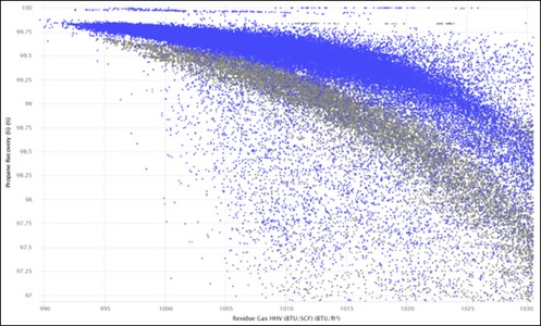
One way to visualize this effect is by plotting the propane recovery of the plant as a function of the residue gas high heating value (HHV). As the plant NGL recovery decreases, the HHV of the residue gas will increase. Ideally, most of the decrease in NGL recovery will be from ethane alone. Except in abnormal pricing conditions, maximum recovery of all other NGL components (C3+) is economically favored. Therefore, an ideal curve should be wide (indicating the ability to achieve both deep recovery and full rejection), while also being flat (increasing ethane rejection levels does not result in significant loss of propane recovery).

FIG. 2 shows propane recovery data for the plant over a 2.5 yr period. The gray data occurred prior to the modifications made to the turboexpander, and the blue data occurred after. Note: the residue gas HHV increases post-modification, and the propane recovery decreases less rapidly, resulting in an incremental increase in propane recovery of 0.5%–1%. Further, the minimum HHV achieved is lower, as indicated by the presence of blue data below 995 Btu/ft3 where gray data does not exist. This indicates that the full recovery condition for the plant shifted to higher levels of NGL recovery. At a large gas plant, this seemingly modest increase in recovery performance can equate to significant increases in cash flow on an annual basis.

FIG. 2

While a dynamic model is not required to troubleshoot this type of problem, its development enabled opportunities such as this to be readily identified. It is not common for an engineer to regularly evaluate plant turboexpander performance against performance curves; however, a continuously-running dynamic simulation can. Because of the insight gained from the model and attention to detail needed to construct it, this long-standing problem could be recognized and corrected, and lost revenue could be reclaimed at no cost to the operator.

Rigorous compression modeling. As previously described, the dynamic model enables the user to simulate a reciprocating compressor by specifying the geometry of the cylinders/stages and the operating speed. The simulator will calculate either suction flow or pressure if the other is specified. Likewise, for centrifugal/axial compressors, the multispeed performance curves can be specified, and the suction pressure will be determined by the simulation instead of being specified by the user. This type of modeling is much more representative of actual plant operations, which better equips the engineer to solve the types of problems encountered during plant optimization exercises and does not require any iteration during the simulation run to arrive at a converged solution.

Rigorous compression modeling: Example 1. For a reciprocating compressor, as the suction pressure is increased, the mass flow through the unit will increase and (typically) required horsepower will increase, as well. To maintain constant flow as the suction pressure is increased, the variable volume pockets (VVP) on the compressor must be opened. VVP’s are devices located on reciprocating compressor cylinders that can be opened or closed to change the capacity of the cylinder. Opening the VVP effectively reduces the capacity of the cylinder, which reduces the flow at a constant suction pressure and speed. Other means exist to change the cylinder capacity, though VVPs are among the most common.

With the VVP opened, to increase the flow back to the original value, the suction pressure must be increased. In steady-state modeling, increasing the suction pressure on a compressor unit operation will decrease power since the inlet mass flow is specified along with the discharge pressure. The only remaining degree of freedom is the unit speed, which the simulation calculates based on the compressor curve or cylinder data. However, in practice, the operator or a controller selects the speed, the discharge pressure is generally fixed (or out of the operator’s control) and the suction pressure/flow is what is varied. To rigorously model the compressor in a way that is useful in a steady-state simulation, the suction pressure of the unit must be changed via a controller unit operation in the simulation until the calculated speed is equal to the desired value. Similar setups are required for centrifugal pumps, turboexpanders, etc. This roundabout way of modeling equipment makes the simulation difficult to understand/maintain and creates model stability issues.

In a dynamic model, this is accomplished without iteration. Cylinder clearance (analogous to VVP opening) can be adjusted in the model and increasing suction pressure on the unit causes the flow to increase and vice versa. The more physically representative modeling can help quantify tradeoffs between various plant operating parameters, including:

1. Residue gas recycle rate: The ability of a plant to recycle lean residue gas back to the inlet is related to the amount of excess residue compressor power. This recycle typically allows for higher NGL recovery levels.
2. Demethanizer pressure: Lower pressures provide higher NGL recovery and mitigate NGL specification concerns for methane and carbon dioxide. This requires more compression power.
3. Plant throughput, which is directly proportional to residue power.
4. Number of compressors in operation.

With the dynamic models in place, regular determination of the minimum number of compression units that should be operating can be completed to ensure that the plant is continuously operating at minimum economical horsepower/MMft3. For instance, a plant may be operating in a condition in which three residue compressors can manage the flowrate required at a relatively high load. Alternatively, four residue compressors can be used at a reduced load. The extra available horsepower can then be used to provide some residue gas recycle to the inlet of the plant or to reduce the demethanizer pressure, both of which increase NGL recovery. However, these benefits come at the cost of increased fuel costs and hours on engines/motors, which incur a maintenance cost. To determine which equipment configuration should be used, a model that can readily and accurately predict the plant performance in the two conditions is required.

Rigorous compression modeling: Example 2. At times, A DCP Midstream plant had been unable to reach its full nameplate capacity of inlet flow. The bottleneck was the residue compression while the plant was operating in rejection mode or at high residue sales line pressure.

Using VVP measurements taken in the field, the model was used to simulate this issue. Performance of the plant could be determined across a range of conditions, including quantifying the tradeoff between plant throughput and NGL recovery. Further, additional configurations of VVP position (load steps) were built into the model to enable the engineer to explore other compressor configurations and observe the impact to performance.

With the model constructed, the following options for the plant could be easily determined:

1. Sacrifice throughput: Operation in full ethane rejection mode and limit the compressors to 100% load. The plant would be limited to ~92% of nameplate capacity. This was the current operating condition.
2. Sacrifice reliability: Operation in full ethane rejection mode, allow the compressors to exceed 100% load and the plant could achieve the full nameplate capacity. The simulation determined that the load in this condition would be ~105%. Although the engines on the compressors can operate up to 110% load, this was deemed unacceptable due to the potential detrimental impact to equipment reliability.
3. Sacrifice propane recovery: Operation in full ethane rejection mode, limit the compressors to 100% load, open the VVPs and the plant could achieve the full nameplate capacity at a higher demethanizer operating pressure. The simulation provided the ability to accurately quantify the suction pressure increase that is required to achieve this condition and how open the VVPs must be, as well. Because the simulation includes a rigorous model of the turboexpander brake compressor and variable pressure drop through the heat exchangers, it could also accurately predict the higher demethanizer operating pressure, resulting in lower propane recovery. The lower propane recovery is a result of the reduction in separation efficiency at high pressure—the ability to selectively reject ethane is limited.
4. Sacrifice full rejection capability: Operation in partial ethane rejection mode, limit the compressors to 100% load, do not open the cylinder VVPs and the plant could achieve the full nameplate capacity. The simulation model could accurately predict the level of ethane recovery required to limit the residue compressor load.

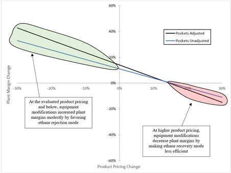
The results from the four cases were provided to DCP Midstream’s finance team to quantify the impact to plant financials. Case 1 was shown not to be an economical option as increasing plant throughput is almost always favorable to any NGL recovery performance. Case 2 was eliminated for reliability reasons. The financial comparison to be made then is between Cases 3 and 4. Pricing sensitivity was completed for these two cases and is shown in FIG. 3 (data has been normalized).

FIG. 3

The analysis showed a modest benefit of adjusting the compressor VVPs for product pricing at or below the pricing at the time of evaluation by favoring ethane rejection mode. Above the baseline product pricing, there was a net-negative impact as ethane recovery mode is favored, and this mode is made less efficient with the proposed equipment modifications. At the time, ethane pricing was depressed but was expected to climb again, so the change was not made. Additionally, the upside in rejection mode was relatively modest. Overall, this analysis enabled DCP Midstream to make an informed decision about the equipment configuration; modifying the compressor VVPs requires a non-trivial amount of work, as well as equipment downtime. It is equally difficult to revert if prices change. By accurately quantifying the plant performance, unnecessary equipment modifications were avoided, and the appropriate business decision could be made.

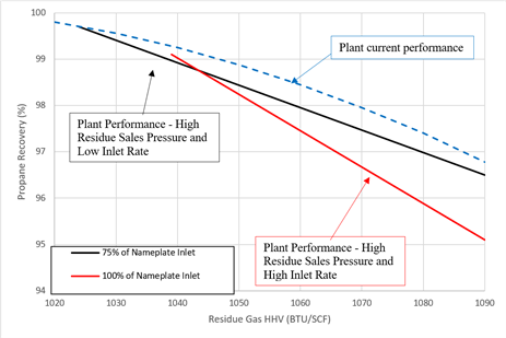
Rigorous compression modeling: Example 3. For another plant, the detailed compressor model was used to quickly solve a different problem. The plant in question typically operated with a residue sales line pressure of no more than 1,000 psig. However, the plant was notified that operating pressures may increase to upwards of 1,200 psig in the future. Given that the plant was already limited on residue compressor capacity, determining the best course of action was required. The dynamic model with multiple load steps built in was able to generate the performance curve shown in FIG. 4 in a matter of hours. This curve was constructed in identical fashion to FIG. 2, showing the propane recovery as the residue gas HHV increases and the plant moves toward ethane rejection mode.

FIG. 4

The modeling results showed that as the residue sales pressure increases, the plant was less able to maintain propane recovery while moving from recovery mode to rejection mode (steeper line), and the maximum NGL recovery level is decreased (left endpoint is higher HHV than other cases). The extent of this effect was dependent on the plant’s inlet rate, which was also quantified in FIG. 4. Because the plant becomes horsepower-limited in this condition, a tradeoff can be made between demethanizer pressure and throughput. Throughput can be maintained, but the demethanizer pressure (and ultimately the residue compressor suction pressure) must be increased. This penalizes NGL recovery performance.

The model also provided information on what VVP adjustments must be made in these cases to accommodate the higher suction/discharge pressures. As described previously, these VVP adjustments must be made to maintain constant flow at increasing suction pressure, thus decreased horsepower.

These results were provided to DCP Midstream’s finance group, which provided financial impact numbers. This enabled the organization to determine if the facility should be operated at the full nameplate capacity, reduced capacity (75% of nameplate) or if a project could be justified to install additional compression to maintain the plants normal/current performance.

 Rigorous compression modeling: Other examples. With the continuously-running models, other compression limitations can be captured in detailed fashion. For instance, some facilities have a dynamic availability of residue compression horsepower depending on ambient temperature. This is typically due to the performance of the cooling of jacket and/or auxiliary water—during the heat of the day, cooling duty may be inadequate, and the load on the unit must be decreased to avoid a high temperature shutdown. This reduction in online horsepower may result in lower throughput or a reduction in plant residue gas recycle, among other possibilities. These changes affect the target operating conditions of the plant, including demethanizer pressure/temperature and refrigeration system performance. If a continuously-running, unsupervised simulation is to provide guidance to an operator on optimized performance for the plant, it must account for these changing limitations. Using the extensive collection of operating data and ambient temperature data, DCP Midstream has been able to quantify the impact on compression load as a function of ambient temperature. This can then be built into a model (the ambient temperature provided as an input in real time), and the targets can adjust as needed to capture this bottleneck. These effects can be similarly captured for other compression bottlenecks, including vibration limitations that affect maximum speed and the effect of changing ambient temperature and evaporator duty on refrigeration systems. GP

Part 2. Part 2 will be featured in the September issue.

NOTES

a AVEVA OSISoft PI System

 

Jake Carrier has been a Process Engineer in DCP Midstream’s operational support and optimization group (ICC) for 5 yr, where he provides technical support for gas plant and field operations teams. His previous experience includes 5 yr working in engineering, procurement and construction as a Process Engineer on projects, including upstream and midstream facilities, sour gas and supercritical carbon dioxide. Mr. Carrier is a graduate of the chemical engineering program at the University of Colorado in Boulder.  

Sjoerd Hoogwater heads the ICC Engineering group at DCP Midstream in Denver, Colorado. He has more than 30 yr of experience in the oil and gas industry. He joined DCP Midstream in 2019 to help expand their process technology and optimization capabilities. Mr. Hoogwater earned an MS degree in chemical engineering from Eindhoven University of Technology in The Netherlands.