Calculate likelihood of piping failure from high-frequency acoustic vibration

The failure of a piping section at the outlet of pressure safety valves (PSVs) and control valves, where significant differential pressure exists, is a common problem, particularly in gas processing. The failure is mostly caused by acoustic induced vibration. High pressure discontinuity generates high vibration and sound levels, causing the failure of the piping system.

The likelihood of failure (LOF) is generally established through the calculation of sound power level (represented as PWL) at the source and at different sections of the downstream piping. It is normally the welded joint that fails due to acoustic excitation. The welded joint can be of any type, including branch connection, welded tee, welded support, etc.

Although there are several modes of acoustic induced vibration failure, this article is restricted to certain types of flow regimes and process connections:

• Flow regime—only gas phase|
• Downstream of PSV
• Blowdown lines—downstream of restriction orifice
• Downstream of control valve
• High pressure venting.

In the case of a control valve, low noise trim is sometimes fitted to avoid the generation of excessive noise. In such cases, the possible reduction of noise level due to trim should be obtained from the valve manufacturer.

High-frequency acoustic excitation. In a gas system, high-frequency acoustic energy¹ can be generated by a pressure-reducing device, such as a relief valve, a blowdown valve, a control valve, etc. Acoustic fatigue is of particular concern, as it tends to affect the safety system.

In addition, the time to failure is short, typically a few minutes or hours, due to the high-frequency response. Along with giving rise to high tonal noise levels external to the pipe, this form of excitation can generate severe high-frequency vibration of the pipe wall. The vibration takes the form of local pipe wall flexure (the shell flexural mode of vibration), resulting in potential high-dynamic stress levels at circumferential discontinuities on the pipe wall, such as small-bore connections, fabricated tees or welded pipe supports.

The high noise levels are generated by high-velocity fluid impingement on the pipe wall, turbulent mixing and, for choked flow, shockwaves downstream of the flow restriction. These effects are functions of pressure drop across the pressure-reducing device and the gas mass flowrate. Typical dominant frequencies associated with high-frequency acoustic excitation are 500 Hz–2,000 Hz.

LOF procedure. The failure possibility is established through the calculation of the likelihood of failure. Corrective action is required at the discontinuities with LOF = 1. Several parameters are estimated for overall calculation of LOF number for various scenarios, as outlined in the following subsections.

Mach number—downstream piping. The Mach number² of the downstream fluid is calculated as shown in Eq. 1:

     PWL design limit. The design limit of sound power level³ is calculated as shown in Eq. 2:

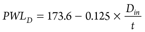If the design limit exceeds the PWL at any point along the pipeline, then the pipeline design is considered to be adequate.

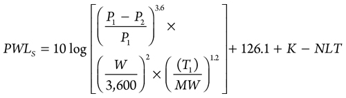
     PWL at source. The PWL at source¹ is calculated using Eq. 3:

where:
      Mach = Mach number
      W = Gas flowrate, kg/hr
      P₁ = Upstream pressure, kPa
      P₂ = Downstream pressure, kPa
      D_in = Pipe inside diameter, mm
      Z = Downstream gas compressibility
      T₁ = Upstream temperature, K
      T₂ = Downstream temperature, K
      MW = Gas molecular weight
      PWL_D = PWL design limit, dB
      PWL_S = PWL at source, dB
      t = Pipe thickness
      K = 0 for subsonic flow, 6 for sonic flow
      NLT = Reduction of noise level (dB) due to low noise trim obtained from the valve                manufacturer.

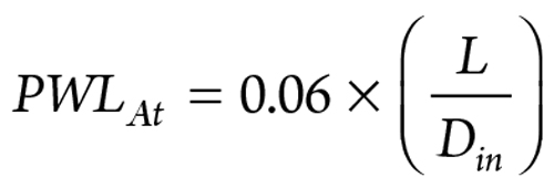
      Attenuation along the pipe. Attenuation along the pipe^2,3 and downstream of the source are estimated as shown in Eq. 4:

where:
      PWL_At = Power level attenuation at distance L, dB
      L = Distance from the source, mm.
      PWL at discontinuity. Actual PWL at downstream discontinuity from a single source¹        is calculated as shown in Eq. 5:

      PWL_dis = PWL_s – PWL_At 

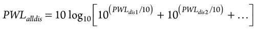
Actual sound power level at downstream discontinuity from multiple sources¹ is calculated as shown in Eq. 6:

where:
      PWL_dis = Power level at discontinuity, single source
      PWL_alldis = Power level at discontinuity, multiple sources.

Example 1. In this example, the PWL at source is estimated for the following PSV design conditions:

• PSV contingency, W = 17,000 kg/hr
• Relief valve set pressure, P₁ = 1,000 kPag
• Relief valve backpressure, P₂ = 0 kPag
• Relieving temperature, T = 30°C
• Vapor molecular weight, MW = 16.4
• Vapor compressibility, Z = 0.97
• Ratio of specific heats, k = 1.3
• Valve discharge coefficient, K_d = 0.975
• Percent overpressure = 10
• Type of PSV = Conventional.

       Solution. The PWL at source is calculated for maximum flow through the PSV, which is
more than the design contingency (17,000 kg/hr). A PSV sizing calculation⁴ is required to establish the maximum flow through the PSV. Critical pressure, P_c, is calculated as shown in Eq. 7:

where relieving pressure, P₁ = 1,201.3 kPa.

Since the critical pressure is greater than the backpressure, the flow will be critical. For critical vapor flow, the orifice area is calculated as shown in Eq. 8:

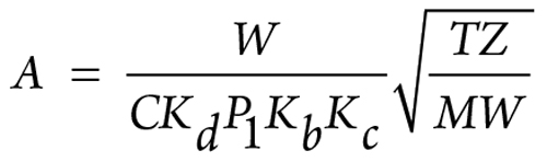where:
      A = Orifice area, mm²
      W = Mass flowrate = 17,000 kg/hr
      C = Coefficient of discharge
      K_d = 0.975
      P₁ = 1201.3 kPa
      K_b = Backpressure correction factor (equal to 1 for a conventional PSV)
      K_c = 1 (no rupture disk)
      T = 303.15 K
      Z = 0.97
      MW = 16.4
      Required orifice = “N”
      Orifice actual area = 2,800 mm².

Note: The coefficient of discharge, C, is calculated as shown in Eq. 9:

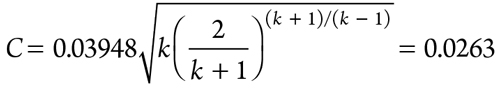      Orifice area, A, is calculated as shown in Eq. 10:

Since the actual orifice area is greater than the calculated orifice area, maximum flow through the orifice will be increased in the same proportion. Therefore, the maximum flowrate through the PSV = 17, 000 × 2,800 ÷ 2,332 = 20,412 kg/hr. The PWL at source is calculated as shown in Eq. 11:

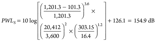The PWL at source calculated using the PSV contingency flow (17,000 kg/hr) is 153.3 dB (1.6 dB less than calculated using the maximum flow through the PSV).

Example 2. In a second example, PSV-A is discharging to atmosphere (FIG. 1), using the following design data estimates:

FIG. 1. Single PSV discharge.

• Section A–B Mach number
• Design limit of sound power level for Section A–B
• Sound power level at Source A
• Attenuation along the Pipe A–B
• Sound power level at discontinuity (Point B).

The design data included:

• Mass flowrate, W = 50,000 kg/hr
• Gas molecular weight, MW = 16.8
• Ratio of gas specific heats = 1.3
• Compressibility, Z = 0.98 (downstream Section A–B)
• Upstream pressure, P₁ = 3401.3 kPa
• Upstream temperature, T₁ = 323.15 K
• Downstream pressure, P₂ = 101.3 kPa
• Downstream temperature, T₂ = 308.15 K
• Section A–B outside diameter = 406.4 mm
• Section A–B thickness = 8.38 mm
• Section A–B length = 10 m.

       Solution. The solution for this example includes five parts:

       1.   Obtain the Mach number with a pipe inner diameter of 389.64 mm, using Eq. 12:

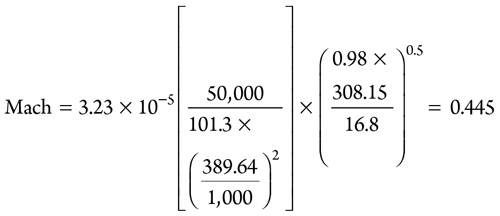       2.   Use Eq. 13 to obtain the design limit of PWL:

       3. Eq. 14 is used to calculate the PWL at source:

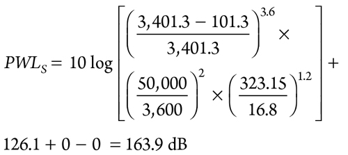             The value of K and NLT are zero.

       4.   Attenuation along pipe Section A–B is calculated with Eq. 15:

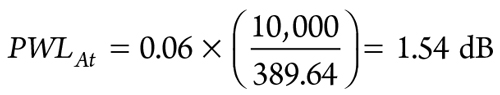       5.   Sound power level at discontinuity (Point B) is obtained, using Eq. 16:

     PWLdis = 163.9–1.54 = 162.4 dB

Example 3. In a third example, PSV-A, PSV-B and PSV-C discharge to a single Point B, as indicated in FIG. 2. The overall PWL at Point B can be estimated, using the following information:

FIG. 2. Multiple PSV discharge.

• Sound power level at Point B due to pipe Section A–B = 162 dB
• Sound power level at Point B due to pipe Section C–B = 165 dB
• Sound power level at Point B due to pipe Section D–B = 167 dB

       Solution. The solution can be estimated using three equations. Consider all three sources, using Eq. 17:

       PWL_alldis = 10 log(10^16.2 + 10^16.5 + 10^16.7) = 169.9 dB

       The PWL for sections C–B and D–B is calculated as shown in Eq. 18:

       PWL_cbdb = 10 log(10^16.5 + 10^16.7) = 169.1 dB 

       The combined PWL, which combines the value derived from Eq. 18 and Section A–B, is calculated as shown in Eq. 19:

       PWL_alldis = 10 log(10^16.91 + 10^16.2 ) = 169.9 dB (as calculated previously) 

Overall design criteria. After the PWL design limit is calculated, the source value and value at discontinuity are established. Design limits are applied to establish the need for further analysis. If PWL_S or PWL_alldis > PWL_D, then the design has failed. In this case, the design must be modified and further analyzed. Several ways exist to modify the design:

• Increase the thickness of the pipe to reduce the design limit
• Reduce the flowrate by increasing the number of PSVs or blowdown valves, which will reduce the PWL at source
• If the flow is choked (Mach number ≥ 1), then the pipe diameter can be increased, which will reduce the PWL at source due to subsonic flow
• The possibility to increase the downstream pressure can be reviewed, which will reduce the PWL at source.

If PWL_S and PWL_alldis < 155, then the design is considered safe. Further analysis is not required for this case.

If the estimated PWL falls outside the aforementioned range, then additional calculations are required to establish the design adequacy. In general, two criteria are used to establish the LOF:

• If the number of cycles to failure ≤ 1E7, then the design is unsafe
• If the number of cycles to failure ≥ 5E8, then the design is safe.

The following procedure is used for the initial estimate, as shown in Eqs. 20–22:

Calculation of the initial number of cycles to failure (N₁) is shown in Eq. 23:

A safety factor of 10 is normally applied to this estimate.

A correction is applied for branch connection (FLM₁) and calculated, using the methodology shown in Eq. 24:

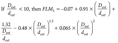Otherwise, FLM₁ = 0.5.

The number of cycles to failure after applying the branch connection correction is calculated, using Eq. 25:

       N₂ = N₁ × FLM₁     

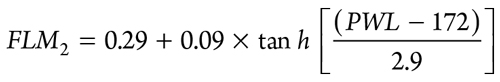
A correction is applied for the type of branch connection (FLM₂) and calculated, using Eqs. 26 and 27. If the connection is a weldolet type fitting (FIG. 3, left):

FIG. 3. Weldolet fitting (left) and welding tee (right).

 

If the connection is a welding tee (FIG. 3, right):

       FLM₂ = 1      

The number of cycles to failure after applying the fitting correction is calculated with Eq. 28:

       N₃ = N₂ × FLM₂ 

A correction is applied for the piping material (FLM₃) and calculated, using the methodology in Eq. 29:

If the piping material is duplex, then

 Otherwise, FLM₃ = 1.

The design number of cycles to failure (N) after applying all correction factors is calculated, using Eq. 30:

        N = N₃ × FLM₃  

where:
     N₁ = Number of cycles to failure, initial estimate
     D_ext = Main pipe external diameter, mm
     d_ext = Branch pipe external diameter, mm
     FLM₁ = Correction factor due to branch connection
     N₂ = Number of cycles to failure after applying branch connection correction factor
     FLM₂ = Correction factor due to fittings
     N₃ = Number of cycles to failure after fitting correction factor
     FLM₃ = Correction factor due to piping material
     N = Design number of cycles to failure
     L_f = Failure factor
     LOF = Likelihood of failure.

Once the design number of cycles to failure is known, the failure factor is calculated as shown in Eq. 31:

     L_f = –0.1303 ln(N) + 3.1 

The design value of failure factor is calculated, using the bases shown in Eq. 32:

      If L_f ≤ 0.0, then L_f = 0
      If L_f ≥ 1.0, then L_f = 1   

Once the value of L_f is known, the likelihood of failure is calculated, using the bases shown in Eq. 33:

      If L_f ≥ 0.5, then LOF = L_f
       If L_f < 0.5, then LOF = 0.29     

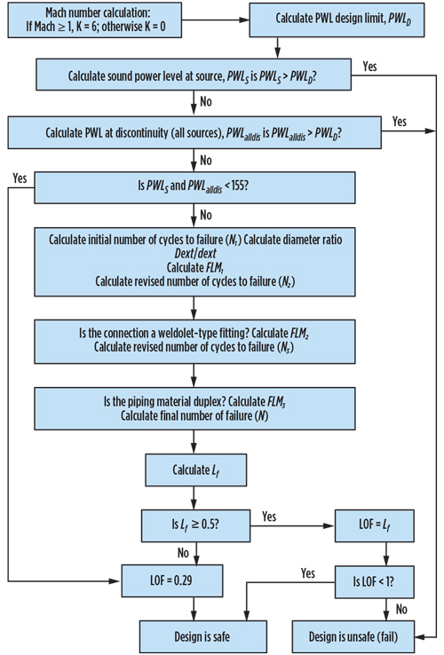
The calculation procedure is further explained in FIG. 4.

FIG. 4. Calculation flowchart.

Example 4. In a fourth example, the blowdown of a compressor package is designed to minimize the blowdown time. A choked flow blowdown is considered (without using any restriction orifices), as shown in FIG. 5. The acoustic induced vibration issue is to be checked for the following conditions:

FIG. 5. Choked flow blowdown (without using any restriction orifice) is considered to minimize the blowdown time.

• Settled out pressure (XV-1 and XV-2 closed) = 10,000 kPag
• Both blowdown valves (DBV-1 and BDV-2) opened at the same time (no delay)
• Settled out temperature = 30°C
• Downstream temperature = –10°C
• Equivalent length of Section A–C = 10 m
• Equivalent length of Section B–C = 10 m
• Equivalent length of Section C–D = 5 m
• Pipe diameter (all sections) = 100 nominal pipe size (NPS), Schedule 120
• Pipe outside diameter = 114.3 mm
• Pipe thickness = 11.31 mm
• Gas molecular weight = 16.8
• Compressibility (discharge) = 0.98.

       Solution. The main problem in this analysis is the calculation of maximum blowdown flow. Since the blowdown is from a source pressure of 10,000 kPag to atmosphere without any restriction orifice, the flow will be choked. The flowrate at choked condition must be estimated.

The volumetric flowrate for compressible fluid^5,6 is calculated as shown in Eq. 34:

where:
      Q = Volumetric flow, Sm³/sec
      Y = Expansion factor
      d = Pipe inside diameter = 0.09168 m
      ∆P = Differential pressure, kPa
      P₁ = Initial pressure = 10,101.3 kPa
      T = Temperature = 303.15K
      S_g = 0.58 (MW = 16.8)
      K = Flow resistance factor.

An estimate of the flow resistance factor considers the following conditions:

• Total equivalent pipe length = 25 m
• Friction factor (fully turbulent flow) = 0.0175
• K (for pipe) = 0.0175 × 25 ÷ 0.09168 = 4.8
• K (entrance) = 1
• K (exit) = 0.5
• Total K = 6.3.

For a compressible gas with a ratio of specific heats in the range of 1.3, the pressure ratio is estimated as shown in Eqs. 35–37:

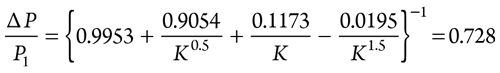      ∆P = 0.728 × 10101.3 = 7353.7 kPa      

      Pressure at Point D = 10,101.3 – 7,353.7 = 2,747.6 kPa 

The expansion factor is calculated, using Eq. 38:

      Y = 0.0415 ln(K) + 0.6097 = 0.686 

The volumetric flow is calculated, using Eq. 39:

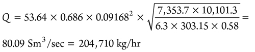The Mach number calculation is shown in Eq. 40:

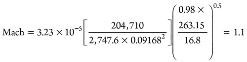Since the Mach number is greater than 1, the value of K in Eq. 3 is 6.

     The PWL design limit is calculated as shown in Eq. 41:

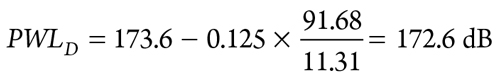     The PWL at source is calculated as shown in Eq. 42:

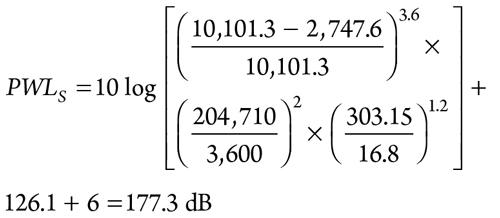     Since PWL_S > PWL_D, the design is not adequate. The design must be modified to avoid acoustic induced vibration failure.

Modification 1. Using the considerations outlined in the previous section, a restriction orifice is added to limit the discharge velocity to Mach 0.7. Since the flow is not choked, the discharge pressure will be close to atmospheric. The estimated flowrate through 100-NPS pipe = 4,700 kg/hr (Mach = 0.7). The flowrate is reduced to approximately 2% of the choked flowrate, which may be too low for this design.

The system adequacy can be checked for this flow condition. The PWL design limit (as calculated previously) = 172.6 dB. The PWL at source calculated for these flow and pressure conditions is shown in Eq. 43:

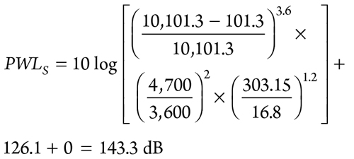PWL at discontinuity is calculated with Eq. 44:

PWL considering all sources is calculated, using Eq. 45:

     PWL_alldis = 10 × log[10^13.68 + 10^13.68 ] = 139.8 dB   

The overall value of PWL at discontinuity is less than the design values and less than 155 dB, which means that the design is adequate.

The conclusion of Modification 1 can be summarized:

• The blowdown rate will decrease significantly; the adequacy of this reduced blowdown rate should be studied further
• With non-choked flow, the design is adequate.

Modification 2. Since Modification 1 results show a significantly reduced blowdown rate, another design option is evaluated considering a higher blowdown rate. The blowdown rate depends on the line size, so a 400-NPS line is considered:

• Line size assumed = 400 NPS
• Line outside diameter = 406.4 mm
• Line thickness = 9.53 mm.

Estimated flow for a velocity of 0.7 Mach = 84,000 kg/hr (i.e., significantly higher than Modification 1).

      The PWL design limit is calculated with Eq. 46:

The PWL at source is calculated, using Eq. 47:

The PWL at discontinuity is calculated with Eq. 48:

The PWL considering all sources is calculated with Eq. 49:

     PWL_alldis = 10 × log[10^16.69 + 10^16.69 ] = 169.8 dB 

Since the PWL considering all sources is greater than the PWL design limit, the design is inadequate.

    The conclusion of Modification 2 can be summarized:

• The blowdown rate increased significantly with respect to Modification 1
• Since the PWL considering all sources is greater than the PWL design limit, the design is not adequate.

Modification 3. Modification 2 can be checked for higher line thickness, as indicated:

• Line size = 400 NPS
• Line outside diameter = 406.4 mm
• Line thickness = 16.66 mm
• Line inner diameter = 373.08 mm.

The estimated flow for a velocity of Mach 0.7 = 79,000 kg/hr (a little less than Modification 2).

       The PWL design limit is calculated with Eq. 50:

The PWL at source is calculated with Eq. 51:

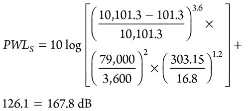The PWL at discontinuity is calculated, using Eq. 52:

The PWL considering all sources is calculated with Eq. 53:

       PWL_alldis = 10 × log[10^16.62 + 10^16.62 ] = 169.2 dB  

In this case, the PWL considering all sources is less than the PWL design limit but greater than 155 dB. Further analysis is required to establish the design adequacy.

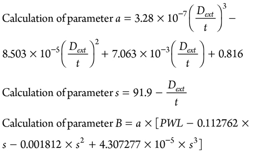
     Calculation parameter a is calculated with Eq. 54:

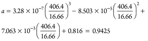Calculation parameter s is calculated, using Eq. 55:

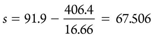Calculation parameter B is calculated with Eq. 56:

B = 0.9425 × [169.2–0.112762 × 67.506–0.001812 × 67.506² + 4.307277 × 10^–5 × 67.506³ ] = 157.04 

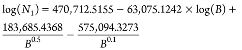
 The initial number of cycles to failure (N₁) is calculated, using Eq. 57:

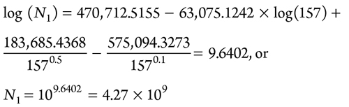The correction for branch connection (diameter ratio = 1) is calculated with Eq. 58:

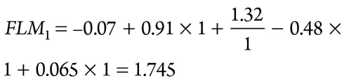For the correction for fittings, assume the fitting is a welding tee; then FLM₂ = 1. For the correction of piping material, assume the piping material is carbon steel; then FLM₃ = 1. The number of cycles after applying all correction factors = 7.46 × 10⁹. After applying a design factor of 10, the design number of cycles to failure is N = 7.46 × 10⁸.

     Calculation of L_f is shown in Eq. 59:

      L_f = –0.1303 × ln(7.46 × 10⁸) + 3.1 = 0.4379 

Since the value of Lf < 0.5, LOF = 0.29; therefore, the design is safe.

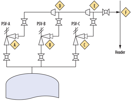
Example 5. In a fifth example, the PSV discharge configuration (FIG. 6) can be used to check for the possibility of acoustic induced vibration failure and if modification is required to avoid AIV failure. The design parameters in TABLE 1 should be used.

FIG. 6. PSV discharge configuration.

 

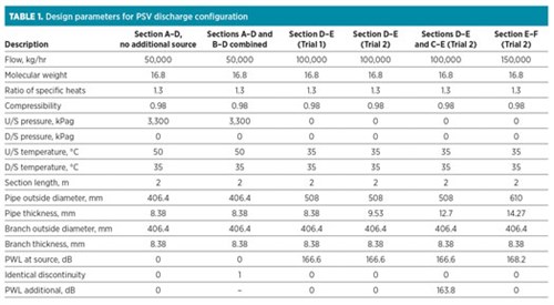The PWL at Point D can be checked for Section A–D without considering additional sources. The source PWL can be calculated from the input parameter—i.e., PWL at source = 0. In this calculation, additional PWL has not been considered. This means that PWL at source will be calculated using Eq. 3; therefore:

• Identical discontinuity = 0
• PWL additional = 0
• Calculated LOF = 0.52
• Health of the joint = OK.

For the calculation of Sections A–D and B–D combined, the input is similar to the previous calculation. However, in this case, additional discontinuity (Section B–D) is added:

• Identical discontinuity = 1
• Calculated LOF = 0.71
• Health of joint = OK.

For the calculation of Section D–E (Trial 1), the main problem is the unavailability of input parameters to calculate the PWL at source. Therefore, the value of the PWL at source must be taken from previous calculations. The section flow is doubled, and a larger pipe (500 NPS) has been considered for this section:

• PWL design limit = 166.3 dB
• PWL at source (used as input) = 166.6 dB (as calculated in previous section)
• Pipe outside diameter = 508 mm
• Pipe thickness = 8.38 mm
• Calculated LOF = 1
• Health of joint = Fail.

      The calculation of Section D–E (Trial 2) features increased pipe thickness:

• Pipe outside diameter = 508 mm
• Pipe thickness = 9.53 mm
• PWL design limit = 167.2 dB
• PWL at source = 166.6 dB
• Calculated LOF = 0.77
• Health of joint = OK.

       In the calculation of Sections D–E and C–E, the source PWL is used as input:

• PWL at source (as before) = 166.6 dB
• Identical discontinuity  = 0
• PWL additional = 163.6 dB (as calculated in Section A–D).

       For Trial 1:

• Pipe outside diameter = 508 mm
• Pipe thickness = 9.53 mm (as before)
• Calculated LOF = 1
• Health of joint = Fail.

      For Trial 2:

• Pipe outside diameter = 508 mm
• Pipe thickness = 12.7 mm (thickness increased)
• Calculated LOF = 0.71
• Health of joint = OK.

      For the calculation of Section E–F:

• PWL at source used as input = 168.2 dB (PWL at discontinuity from previous calculation)
• Line outside diameter = 610 mm
• Line thickness = 14.27 mm
• Calculated LOF = 0.75
• Health of joint = OK.

Recommendations. A systematic analysis is required to establish the possibility of acoustic induced vibration failure. The analysis must be carried out for each section of the system, keeping in mind that the result of one section may influence the outcomes of associated sections.

It is always recommended to conduct a detailed study for acoustic induced vibration failure where significant pressure discontinuity exists. The study here is recommended for greenfield developments and for any existing plant. GP

LITERATURE CITED

1. Energy Institute, Guidelines for the Avoidance of Vibration Induced Fatigue Failure in Process Pipework, 2nd Ed., Energy Institute, London, UK, 2008.
2. API Standard 521, “Pressure-relieving and depressuring systems,” 5th Ed., American Petroleum Institute, Washington D.C., 2007.
3. NORSOK Standard L-002, “Piping system layout, design and structural analysis, 3rd Ed., Standards Norway, 2009.
4. API Standard 520, “Sizing, selection and installation of pressure-relieving devices in refineries, Part 1: Sizing and selection,” 8th Ed., American Petroleum Institute, Washington D.C., 2008.
5. Crane Technical Paper No. 410, “Flow of fluids through valves, fittings and pipe, metric edition—SI units,” Crane Co., 1995.
6. Datta, A., Process Engineering and Design Using Visual Basic, 2nd Ed., CRC Press, New York, New York, 2014.